04. What is Batch Normalization?
What is Batch Normalization?
Batch normalization was introduced in Sergey Ioffe's and Christian Szegedy's 2015 paper Batch Normalization: Accelerating Deep Network Training by Reducing Internal Covariate Shift. The idea is that, instead of just normalizing the inputs to the network, we normalize the inputs to every layer within the network.
Batch Normalization
It's called "batch" normalization because, during training, we normalize each layer's inputs by using the mean and standard deviation (or variance) of the values in the current batch. These are sometimes called the batch statistics.
Specifically, batch normalization normalizes the output of a previous layer by subtracting the batch mean and dividing by the batch standard deviation.
Why might this help? Well, we know that normalizing the inputs to a network helps the network learn and converge to a solution. However, a network is a series of layers, where the output of one layer becomes the input to another. That means we can think of any layer in a neural network as the first layer of a smaller network.
Normalization at Every Layer
For example, imagine a 3 layer network.
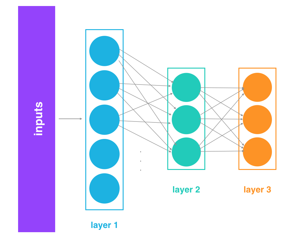
3 layer network
Instead of just thinking of it as a single network with inputs, layers, and outputs, think of the output of layer 1 as the input to a two layer network. This two layer network would consist of layers 2 and 3 in our original network.
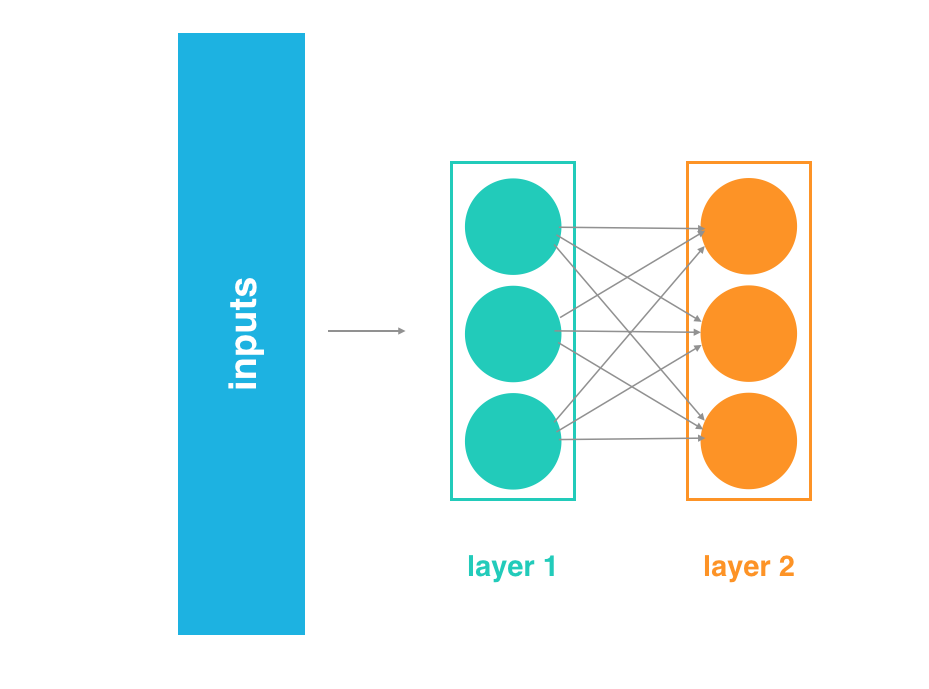
2 layer network
Likewise, the output of layer 2 can be thought of as the input to a single layer network, consisting only of layer 3.
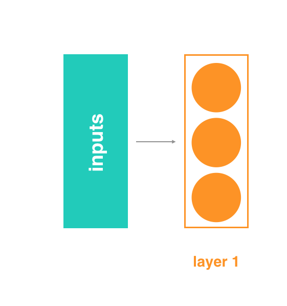
One layer network
When you think of it like this - as a series of neural networks feeding into each other - then it's easy to imagine how normalizing the inputs to each layer would help. It's just like normalizing the inputs to any other neural network, but you're doing it at every layer (sub-network).
Internal Covariate Shift
Beyond the intuitive reasons, there are good mathematical reasons to motivate batch normalization. It helps combat what the authors call internal covariate shift.
In this case, internal covariate shift refers to the change in the distribution of the inputs to different layers. It turns out that training a network is most efficient when the distribution of inputs to each layer is similar!
And batch normalization is one method of standardizing the distribution of layer inputs. This discussion is best handled in the paper and in Deep Learning, a book you can read online written by Ian Goodfellow, Yoshua Bengio, and Aaron Courville. Specifically, check out the batch normalization section of Chapter 8: Optimization for Training Deep Models.
The Math
Next, let's do a deep dive into the math behind batch normalization. This is not critical for you to know, but it may help your understanding of this whole process!
Getting the mean and variance
In order to normalize the values, we first need to find the average value for the batch. If you look at the code, you can see that this is not the average value of the batch inputs, but the average value coming out of any particular layer before we pass it through its non-linear activation function and then feed it as an input to the next layer.
We represent the average as mu_B
We then need to calculate the variance, or mean squared deviation, represented as
If you aren't familiar with statistics, that simply means for each value x_i, we subtract the average value (calculated earlier as mu_B), which gives us what's called the "deviation" for that value. We square the result to get the squared deviation. Sum up the results of doing that for each of the values, then divide by the number of values, again m, to get the average, or mean, squared deviation.
Normalizing output values
Once we have the mean and variance, we can use them to normalize the values with the following equation. For each value, it subtracts the mean and divides by the (almost) standard deviation. (You've probably heard of standard deviation many times, but if you have not studied statistics you might not know that the standard deviation is actually the square root of the mean squared deviation.)
Above, we said "(almost) standard deviation". That's because the real standard deviation for the batch is calculated by
but the above formula adds the term epsilon before taking the square root. The epsilon can be any small, positive constant, ex. the value 0.001. It is there partially to make sure we don't try to divide by zero, but it also acts to increase the variance slightly for each batch.
Why add this extra value and mimic an increase in variance? Statistically, this makes sense because even though we are normalizing one batch at a time, we are also trying to estimate the population distribution – the total training set, which itself an estimate of the larger population of inputs your network wants to handle. The variance of a population is typically higher than the variance for any sample taken from that population, especially when you use a small sample size (a small sample is more likely to include values near the peak of a population distribution), so increasing the variance a little bit for each batch helps take that into account.
At this point, we have a normalized value, represented as
But rather than use it directly, we multiply it by a gamma value, and then add a beta value. Both gamma and beta are learnable parameters of the network and serve to scale and shift the normalized value, respectively. Because they are learnable just like weights, they give your network some extra knobs to tweak during training to help it learn the function it is trying to approximate.
We now have the final batch-normalized output of our layer, which we would then pass to a non-linear activation function like sigmoid, tanh, ReLU, Leaky ReLU, etc. In the original batch normalization paper, they mention that there might be cases when you'd want to perform the batch normalization after the non-linearity instead of before, but it is difficult to find any uses like that in practice.